5 Import/Export

Objective:
- Learn how to import (read.csv(), read.delim()) and export tabular data (write.csv(), write.delim()) - Learn how to plot graphs using base R

We will cover:

• use data sets provided by R
• how to create a new directory/folder using dir.create()
  
• open several graphics windows
  
• save plots to file

5.1 Export Tables

** Tips for Preparing Data**

• first row = column headers (variables) and first column = row names (observations) Row and column names
  
• should be unique
  
• shouldn’t begin with a number
  
• no special symbols (except underscore)
  
• avoid blank spaces
  
• avoid blank rows and comments
  
• use the four digit format for date: Good: 01/01/2016. Bad: 01/01/16

In Excel, save your file into .txt (tab-delimited text file) or .csv (comma separated value file) format.

Working with txt and csv files - R has built-in datasets that we may use (see datasets with data() command)

# Call data into environment with data("dataset")
# Loading DNase data
data("DNase")
# Get more info using ?
# ?DNase
# See first 10 rows with head()
head(DNase, n = 10) 

##    Run       conc density
## 1    1 0.04882812   0.017
## 2    1 0.04882812   0.018
## 3    1 0.19531250   0.121
## 4    1 0.19531250   0.124
## 5    1 0.39062500   0.206
## 6    1 0.39062500   0.215
## 7    1 0.78125000   0.377
## 8    1 0.78125000   0.374
## 9    1 1.56250000   0.614
## 10   1 1.56250000   0.609

# basic stats with summary()
summary(DNase)

##       Run          conc             density      
##  10     :16   Min.   : 0.04883   Min.   :0.0110  
##  11     :16   1st Qu.: 0.34180   1st Qu.:0.1978  
##  9      :16   Median : 1.17188   Median :0.5265  
##  1      :16   Mean   : 3.10669   Mean   :0.7192  
##  4      :16   3rd Qu.: 3.90625   3rd Qu.:1.1705  
##  8      :16   Max.   :12.50000   Max.   :2.0030  
##  (Other):80

# unique values of a vector with unique()
unique(DNase$Run)

##  [1] 1  2  3  4  5  6  7  8  9  10 11
## Levels: 10 < 11 < 9 < 1 < 4 < 8 < 5 < 7 < 6 < 2 < 3

R base functions for exporting/writing/saving data: * write.table() - exporting any tabular data to “.txt” file * write.csv() - comma separated values,“.csv” file

variations when comma (,) is used as decimal points instead of periods (.): write.csv2()

Arguments:
- file = absolute/local file paths with name of file - sep = field seperators (sep argument) - character(s), controls the way splits a data table into fields/cells
- header = logical for column names
- row.names = vector of row names or number/name of column which contains the row names

# Create a Data folder
dir.create("Data")

## Warning in dir.create("Data"): 'Data' already exists

# Write data to txt file: tab separated values
# sep = "\t"
write.table(DNase, file = "Data/DNase.txt", sep = "\t", row.names = FALSE) #"\t" means "tab"

# Write data to csv files:
# decimal point = "." and value separators = comma (",")
write.csv(DNase, file = "Data/DNase.csv")

# Write data to csv files:
# decimal point = comma (",") and value separators = semicolon (";")
# write.csv2(DNase, file = "DNase.csv")

5.2 Import Tables

R base functions for importing data

• read.table() - reading any tabular data
  
• read.delim() - reading tab-separated value files (.txt)
  
• read.csv() - comma separated value files (.csv)

variations when comma (,) is used as decimal points: read.delim2(), read.csv2()

• file = absolute/local file paths with name of file, file.choose() to choose interactively, internet address e.g. “http://www.sthda.com/upload/boxplot_format.txt”

# Read tabular data into R
# file.choose() allows you to interactively pick a data file
# df <- read.table(file.choose(), header = FALSE, sep = "\t", dec = ".")
# Read "comma separated value" files (".csv")
filename <- "Data/DNase.csv"
df <- read.csv(filename, header = TRUE)
# Read TAB delimited files
df2 <- read.delim(file = "Data/DNase.txt", header = TRUE, sep = "\t", dec = ".")
# Note to save into an object, we must assign to variable!

Working with Excel files * openxlsx package
* readxl package

Note: install libraries/packages in R using install.packages(“package_name”). Load intro environment before using with library(package_name)

Writing Data From R to Excel Files (xls|xlsx)

# # install.packages("openxlsx")
# 
# library("openxlsx") # or require("openxlsx")
# # Write the first 10 rows in a new workbook
# write.xlsx(DNase[1:10,], file = "Data/DNase.xlsx", sheetName = "DNase 1", append = FALSE)
# # Add a second data set in a new worksheet with first and third column
# write.xlsx(DNase[,c(1,3)], file = "Data/DNase.xlsx", sheetName = "DNase 2", append = TRUE)

Reading data From Excel Files (xls|xlsx) into R

# # Use openxlsx package
# my_data <- read.xlsx("Data/DNase.xlsx", sheetIndex = 1) 

Using R data format: RDATA and RDS

• Save/load variables, user-made functions and data Saving objects
• Save one object to a file: saveRDS(object, file)
• Save multiple objects to a file: save(data1, data2, file)
• Save your entire workspace (all objects): save.image() Loading objects
• readRDS(rds_file), load(RData_file)

# # Save a single object to a file
# saveRDS(DNase, "Data/DNase.rds")
# # Restore it under a different name
# my_data <- readRDS("Data/DNase.rds")
# # Save multiple objects
# save(DNase, my_data, file = "Data/data.RData")
# # To load the data again
# load("Data/data.RData")
# # Saving and restoring your entire workspace:
# # Save your workspace
# save.image(file = "Data/my_work_space.RData")
# # Load the workspace again
# load("Data/my_work_space.RData")

Consider using readr package * Reading lines from a file: read_lines()
* readr functions for writing data: write_tsv(), write_csv()
* readr for reading/writing txt|csv files: read_tsv(), read_csv(), etc

5.3 Graphing with base R

• Now that we can import our data, we can learn how to plot it.
• The purpose of base R plots is to analyze our data, not as elegant for publication purposes

plot() - generic function, meaning it can work with different types of objects
- plot() function can be used to plot 2 variables (of equal length) plot(x, y, type=…) Arguments x and y = the coordinates of points to plot type = the type of graph to create, possible values: “p” - points - scatter plot
“l” - lines
“b” - both points and lines
“c” - empty points joined by lines
“o” - overplotted points and lines
“s” and “S” - stair steps
“h” - histogram-like vertical lines
“n” - does not produce any points or lines
main = Title for plot
xlab = Title for x axis
ylab = Title for y axis

• You can specify fonts, colors, line styles, axes, reference lines, etc. by adding graphical parameters (cex, col, lwd, etc) Read more: https://www.statmethods.net/advgraphs/parameters.html

• Combine plots using par()
  Read more: https://www.statmethods.net/advgraphs/layout.html

# You can plot all pairs of variables in one graph
plot(DNase)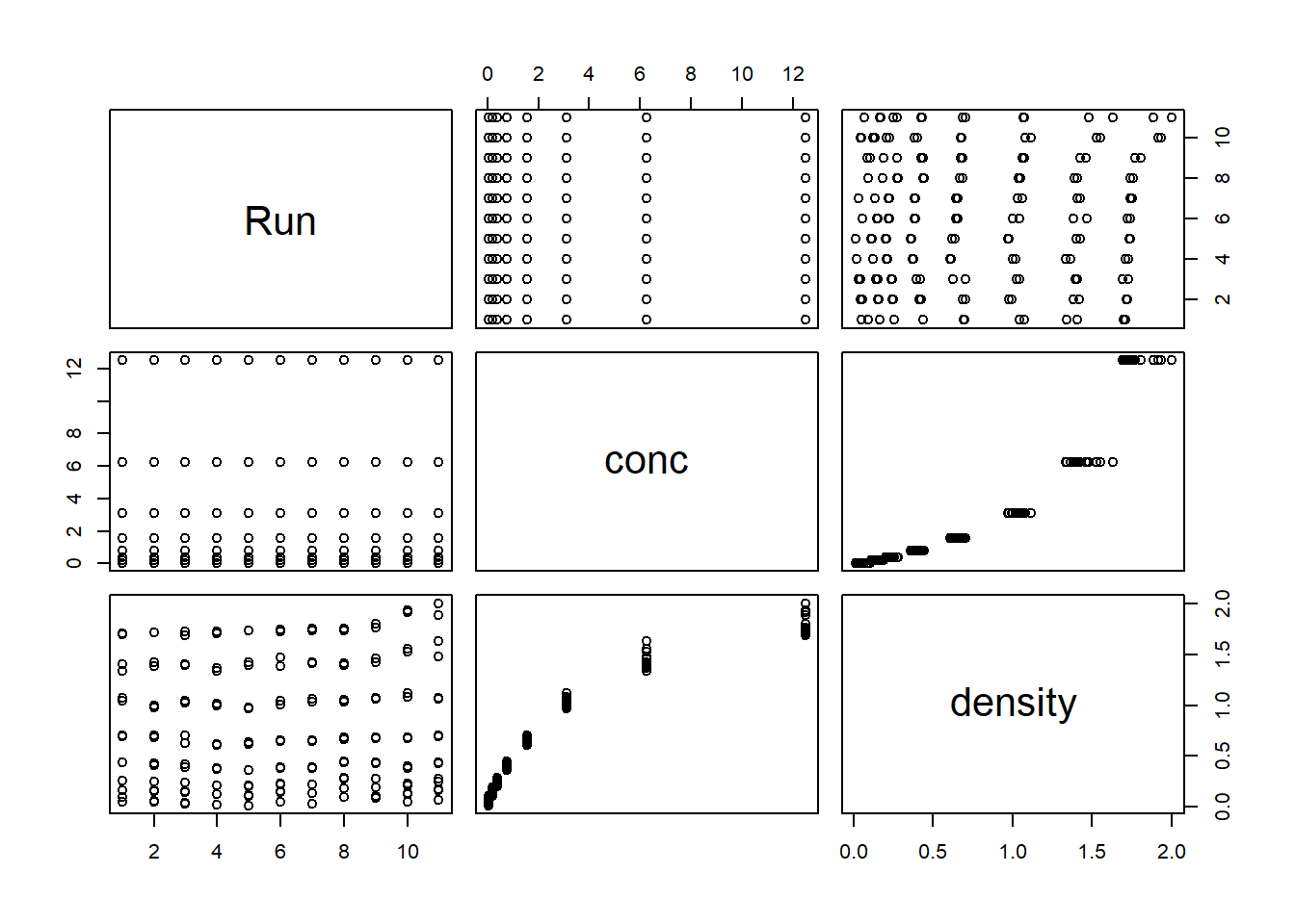

# You can also specify vectors to plot
conc <- DNase$conc; dens <- DNase$density
plot(x = conc, y = dens, type ="p")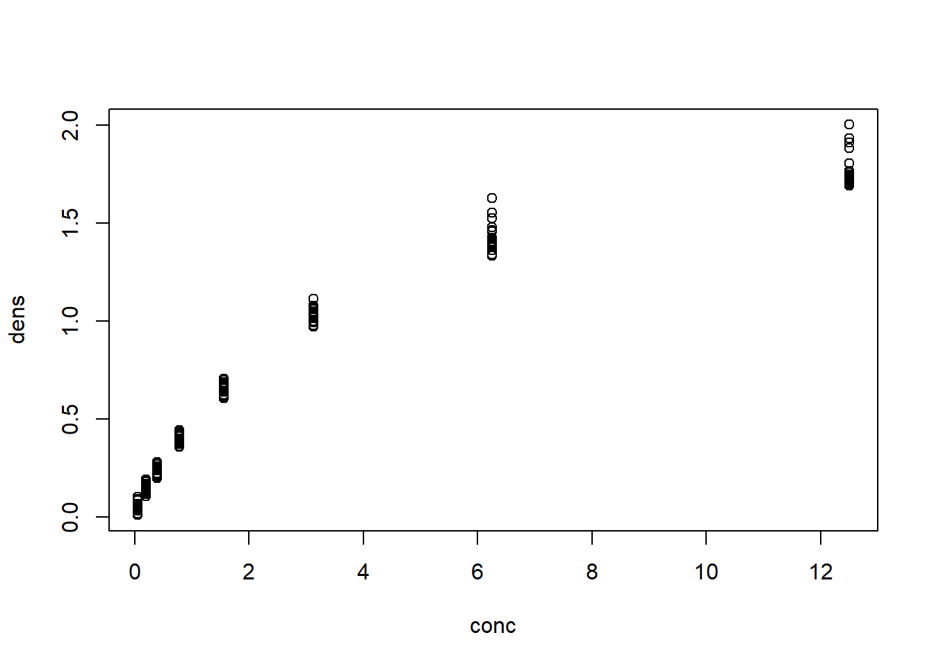 

plot(x = conc, y = dens, type ="h")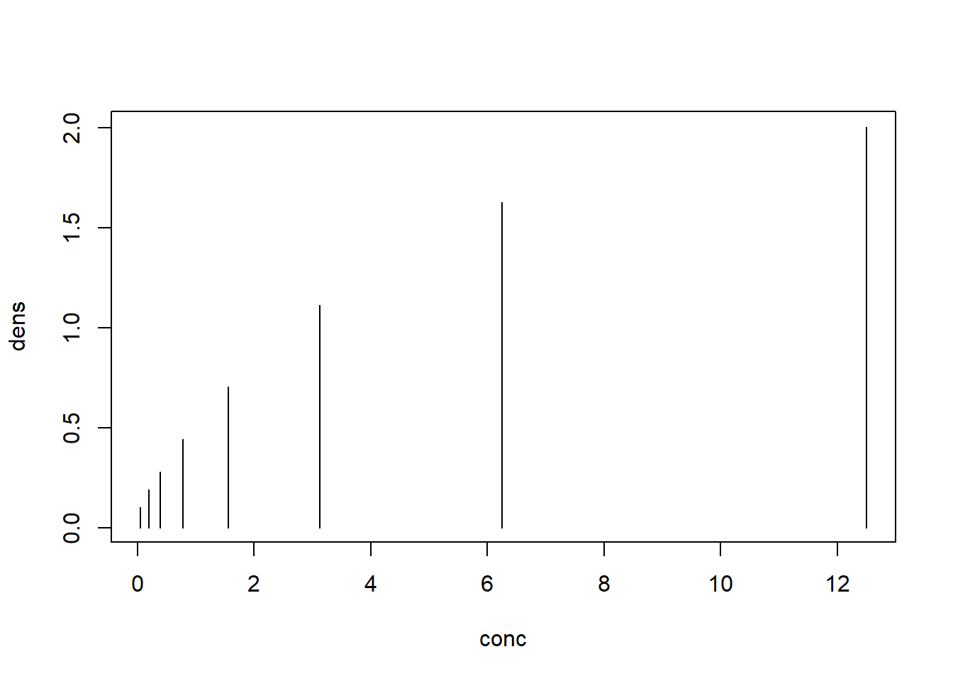

plot(x = conc, y = dens, type ="s")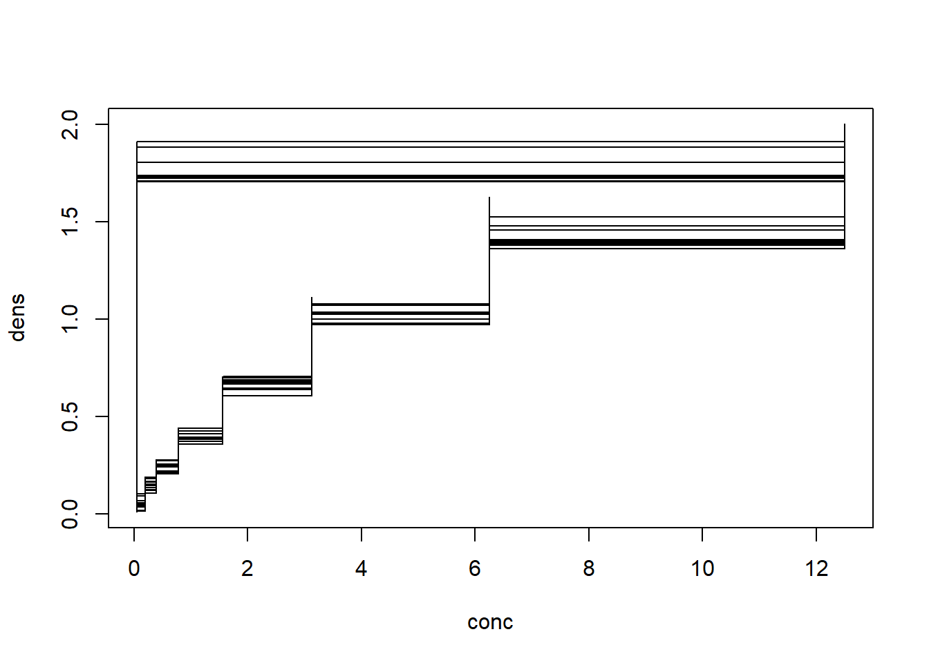

# Add title 
plot(x = conc, y = dens, type ="h",
     col = "red", # colour of line
     lwd = 3, # width of line
     xlab = "Conc", ylab = "Density", # x, y axis labels
     main = "ELISA Assay of DNase") # title for plot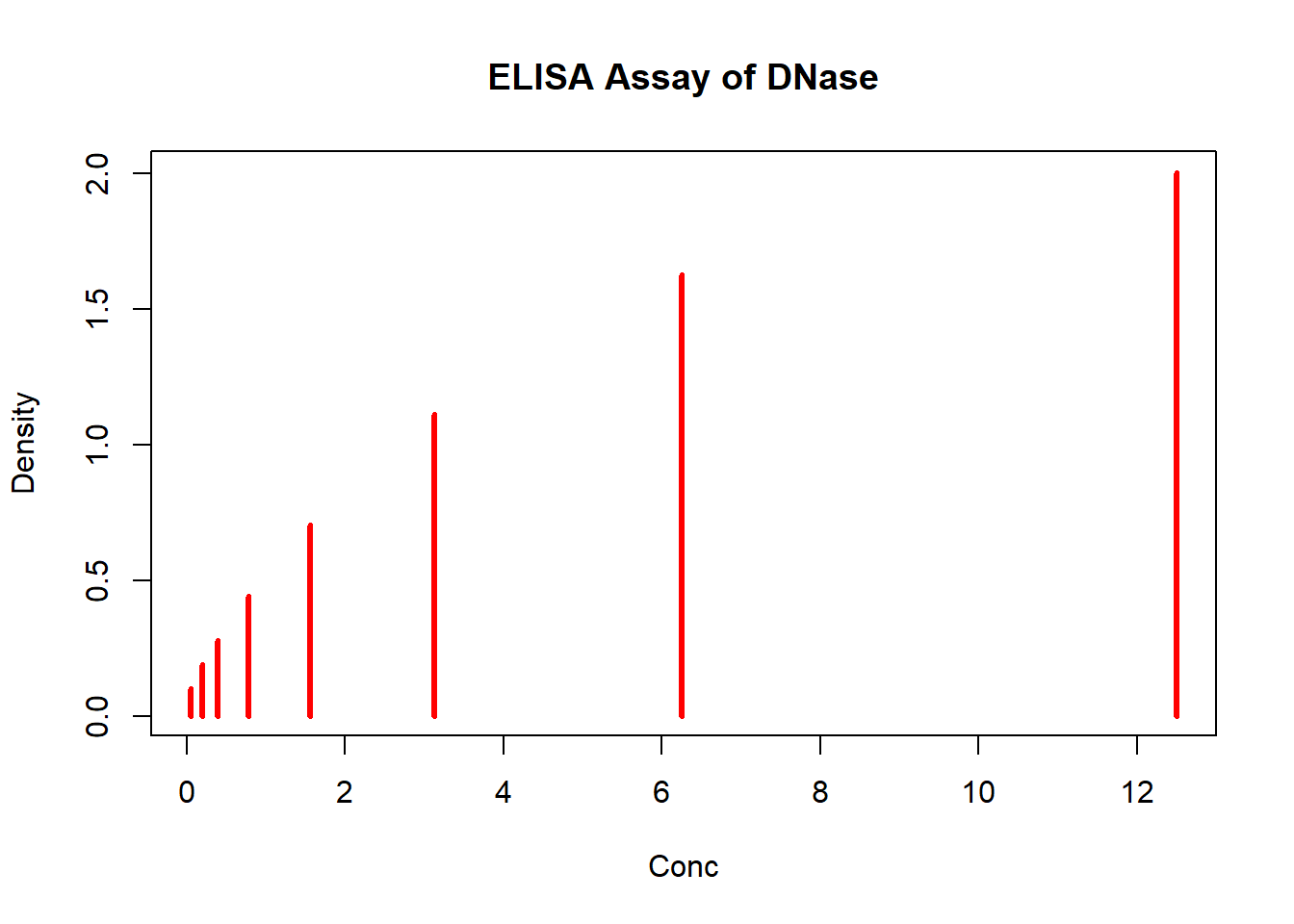

Tip: Open graphics windows before calling plot() to view larger plot/several graphs at once

Function - Platform In Windows, windows() or win.graph() In Unix, X11() In Mac, quartz() or x11()

# windows()
x <- seq(-pi,pi, by = 0.1)
plot(x, sin(x), main="The Sine Function")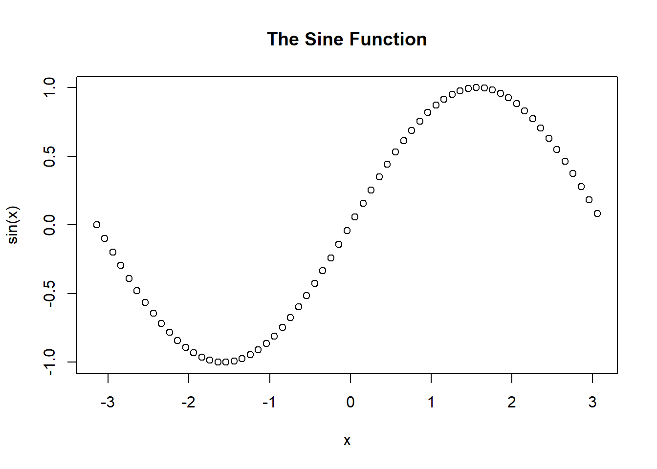

Plot line graph with regression

• Linear regression: statistical analysis technique used to determine the extent to which there is a linear relationship between a dependent variable and one or more independent variables

• create simple regression using lm() or “linear model” function
  

• 2 common parameters:
  + formula: describes the model with the format “Y-var ~ X-var”, where Y-var is the dependent variable and X-var is independent variable
  + data: the variable that contains the dataset
  

• summary() is used to find the intercept and coefficients (under “Estimate”), R^2 and p-value
  Recall: y = mx + b, where m is c

Read more: https://www.r-bloggers.com/r-tutorial-series-simple-linear-regression/

# Plot 
plot(DNase$conc, y <- DNase$density, 
     type = "p", # line graph
     col = "red", # colour of line
     lwd = 3, # width of line
     xlab = "Concentration", # x axis label
     ylab = "Density", # y axis label
     main = "ELISA assay of DNase") # title of plot
# Make a linear model with the density and concentration variables
fit <- lm (density ~ conc, data = DNase) 
fit

## 
## Call:
## lm(formula = density ~ conc, data = DNase)
## 
## Coefficients:
## (Intercept)         conc  
##      0.2949       0.1366

# Get statistics
summary(fit)

## 
## Call:
## lm(formula = density ~ conc, data = DNase)
## 
## Residuals:
##      Min       1Q   Median       3Q      Max 
## -0.30901 -0.19640 -0.03957  0.19498  0.48056 
## 
## Coefficients:
##             Estimate Std. Error t value Pr(>|t|)    
## (Intercept)  0.29488    0.02072   14.23   <2e-16 ***
## conc         0.13657    0.00406   33.63   <2e-16 ***
## ---
## Signif. codes:  0 '***' 0.001 '**' 0.01 '*' 0.05 '.' 0.1 ' ' 1
## 
## Residual standard error: 0.2181 on 174 degrees of freedom
## Multiple R-squared:  0.8667, Adjusted R-squared:  0.8659 
## F-statistic:  1131 on 1 and 174 DF,  p-value: < 2.2e-16

# Add a line to the plot (new layer)
abline(fit)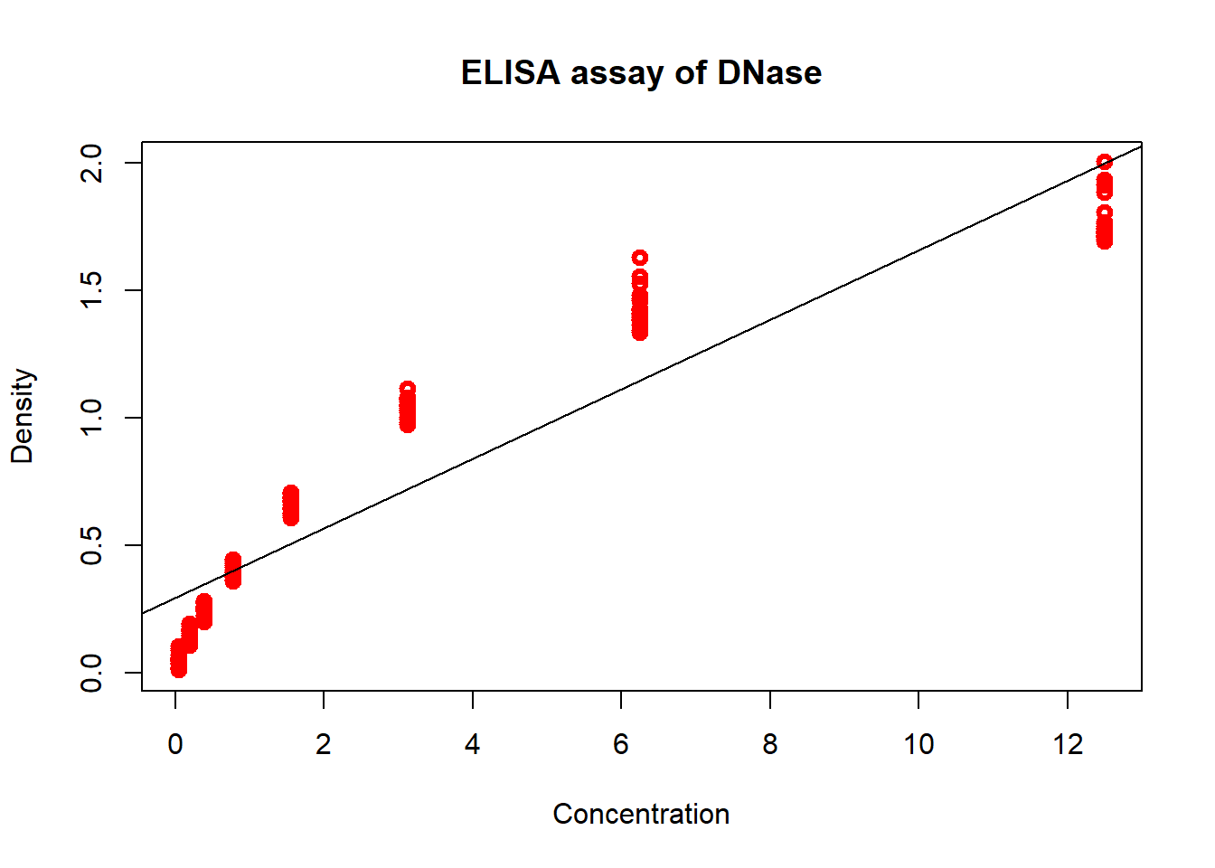

# Add text to the plot (new layer)
# text()

Make a basic histogram of a numeric vector using hist()

• ref: https://rstudio-pubs-static.s3.amazonaws.com/7953_4e3efd5b9415444ca065b1167862c349.html
  
• Histograms: show frequencies for ranges of values

hist(DNase$density)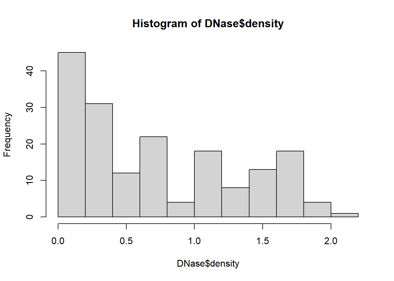

Saving to File

1 - Plot by exporting using “Export” in plot panel (bottom-right pane) or in window menu 2 - Plot by opening a file connection Format: type_of_file(“filename”) pdf(rplot.pdf): pdf file png(rplot.png): png file jpeg(rplot.jpg): jpeg file postscript(rplot.ps): postscript file bmp(rplot.bmp): bmp file win.metafile(rplot.wmf): windows metafile Note: Use “dev.off()” to close the connection after plotting

# Create 2 vectors with 10 elements/values
TEN_Random <- runif(10, 0.0, 1.0)
TEN_sequence <- seq(from = 1, to = 30, length.out = 10)
# Make the second value missing in y 
TEN_sequence[2] <- NA
# Create a "Plots" directory in your current working directory
dir.create("Plots")

## Warning in dir.create("Plots"): 'Plots' already exists

# Save to png file
png("Plots/plot.png") # open "device" connection
plot(x = TEN_sequence, y = TEN_Random, xlab = "Index", ylab = "Random values") # plot
dev.off() #close connection

## png 
##   2

Create an editable graph from R using ReporteRs package

• Editable vector graphics can be created and saved in a Microsoft document
• Read here: http://www.sthda.com/english/wiki/create-an-editable-graph-from-r-software

5.4 Practice

The “women” data set in R gives the average heights and weights for American women aged 30 to 39.
a) Print the first 15 rows to the console. (Hint: use the “n” argument in head() function)
b) Create a folder called “Data Sets” in your current working directory.
c) Write the women data frame as a csv file to the Data Sets folder (exclude row names).
d) Read this file back into R and assign it to a variable called “women.df”.
e) Plot a histogram of the heights column.
f) Find the mean and standard deviation of heights (Recall: vectors tutorial)
g) print the variables from f) in a statement “The mean and standard deviation of the heights is __ and __” (Hint: use sprintf() or paste() )
h) Plot a scatter plot, where x = height and y = weight. Relabel x and y axes to “Height (in)” and “Weight (lbs)” respectively.
i) Save f) to a jpeg file.

Solution

data("women")
# a) Print using head()
head(women, n = 15)

##    height weight
## 1      58    115
## 2      59    117
## 3      60    120
## 4      61    123
## 5      62    126
## 6      63    129
## 7      64    132
## 8      65    135
## 9      66    139
## 10     67    142
## 11     68    146
## 12     69    150
## 13     70    154
## 14     71    159
## 15     72    164

# b) Create a folder using dir.create()
dir.create("Data Sets")

## Warning in dir.create("Data Sets"): 'Data Sets' already exists

# c) Write to csv using write.csv()
write.csv(x = women, file = "Data sets/women.csv", row.names = F)
# d) Read using read.csv()
women.df <- read.csv(file = "Data sets/women.csv")
# e) Plot histogram using hist()
hist(women.df$height)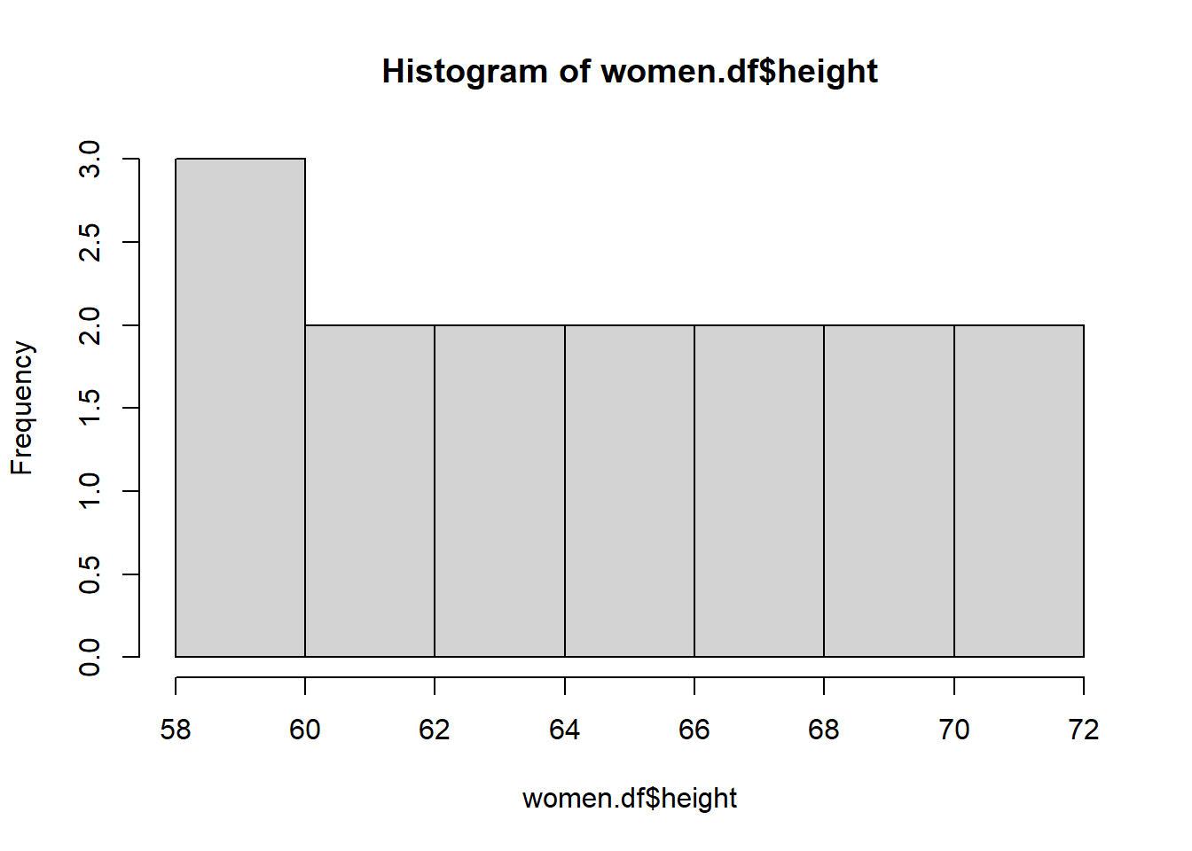

# f) Find mean using mean() and standard deviation using sd()
mean.hts <- mean(women.df$height)
sd.hts <- sd(women.df$weight)
# g) Print
sprintf("The mean and standard deviation of the heights is %s and %s", mean.hts, sd.hts)

## [1] "The mean and standard deviation of the heights is 65 and 15.4986942614378"

paste("The mean of the heights is ", mean.hts, " and ", sd.hts, sep = "")

## [1] "The mean of the heights is 65 and 15.4986942614378"

# h) Plot using plot()
plot(x=women.df$height, y=women.df$weight, xlab = "Height (in)", ylab = "Weight (lbs)", main = "Avg Heights and Weights for American Women 30-39")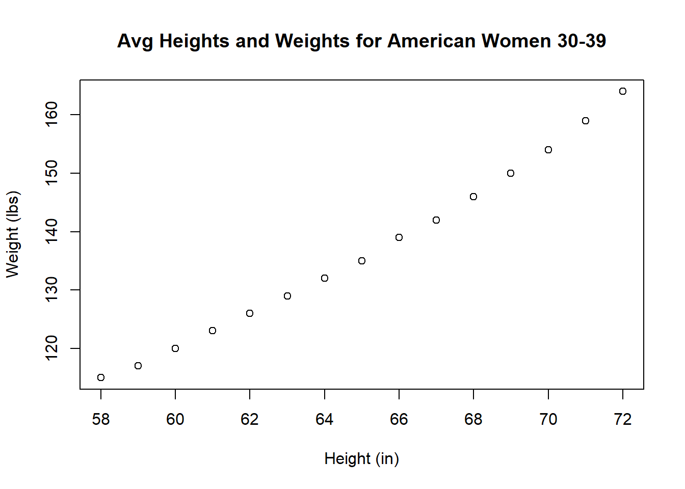

# i) Save as jpeg
jpeg(filename = "heights_vs_weights.jpeg")
plot(x=women.df$height, y=women.df$weight, xlab = "Height (in)", ylab = "Weight (lbs)", main = "Avg Heights and Weights for American Women 30-39")
dev.off()

## png 
##   2